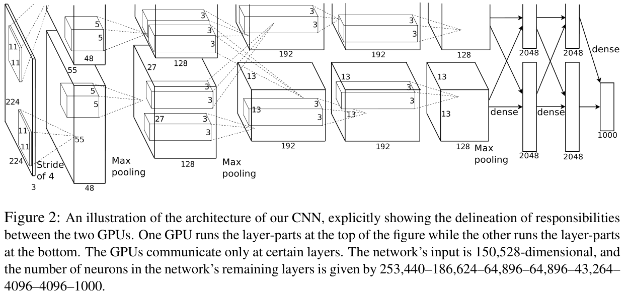
AlexNet 网络模型搭建 根据 ImageNet Classification with Deep Convolutional Neural Networks 论文中的文字描述和图标信息,可以得到 AlexNet 模型(忽略 batch_size )如下
layer_name out_size out_channel kernel_size padding stride Input 224*224 3 None None None Conv1 55*55 96 11 2 4 Maxpool1 27*27 96 3 0 2 Conv2 27*27 256 5 2 1 Maxpool2 13*13 256 3 0 2 Conv3 13*13 384 3 1 1 Conv4 13*13 384 3 1 1 Conv5 13*13 256 3 1 1 Maxpool3 6*6 256 3 0 2 FC1 4096 1 None None None FC2 4096 1 None None None FC3 1000 1 None None None
据此可搭建网络模型
1
2
3
4
5
6
7
8
9
10
11
12
13
14
15
16
17
18
19
20
21
22
23
24
25
26
27
28
29
30
31
32
33
34
35
36
37
38
39
40
41
42
43
44
45
46
47
48
49
50
51
class AlexNet_Paper (nn.Module): def __init__ (self, input_channel=3 , num_classes=1000 ): super (AlexNet_Paper, self ).__init__() self .conv1 = nn.Sequential( nn.Conv2d(in_channels=input_channel, out_channels=96 , kernel_size=11 , stride=4 , padding=2 ), nn.ReLU(inplace=True ), nn.MaxPool2d(kernel_size=3 , stride=2 ), ) self .conv2 = nn.Sequential( nn.Conv2d(in_channels=96 , out_channels=256 , kernel_size=5 , padding=2 ), nn.ReLU(inplace=True ), nn.MaxPool2d(kernel_size=3 , stride=2 ), ) self .conv3 = nn.Sequential( nn.Conv2d(in_channels=256 , out_channels=384 , kernel_size=3 , padding=1 ), nn.ReLU(inplace=True ), ) self .conv4 = nn.Sequential( nn.Conv2d(in_channels=384 , out_channels=384 , kernel_size=3 , padding=1 ), nn.ReLU(inplace=True ), ) self .conv5 = nn.Sequential( nn.Conv2d(in_channels=384 , out_channels=256 , kernel_size=3 , padding=1 ), nn.ReLU(inplace=True ), nn.MaxPool2d(kernel_size=3 , stride=2 ), ) self .fc1 = nn.Sequential( nn.Flatten(), nn.Linear(6 * 6 * 256 , 4096 ), nn.ReLU(inplace=True ), nn.Dropout(p=0.5 ), ) self .fc2 = nn.Sequential( nn.Linear(4096 , 4096 ), nn.ReLU(inplace=True ), nn.Dropout(p=0.5 ), ) self .fc3 = nn.Sequential( nn.Linear(4096 , num_classes), ) def forward (self, x ): x = self .conv1(x) x = self .conv2(x) x = self .conv3(x) x = self .conv4(x) x = self .conv5(x) x = self .fc1(x) x = self .fc2(x) x = self .fc3(x) return x
各层输出 size 计算 Conv 层的输出 size 计算公式
设输入 size 为 i * i ,卷积核 size 为 k * k ,步长为 s ,边缘填充为 p ,输出 size 为 o * o
$$o = \frac{i-k+2*p}{s}+1$$
Maxpool 层的 size 计算公式
设输入 size 为 i * i ,池化核 size 为 k * k ,步长为 s ,输出 size 为 o * o
$$o = \frac{i-k}{s}+1$$
AlexNet 输入 size 问题 AlexNet 输入的图像 size 在论文中多处均描述为 224*224 ,Maxpool1 层输入的 size 在论文 Figure2 中描述为 55*55
image.png The first convolutional layer filters the 224×224×3 input image with 96 kernels of size 11×11×3 with a stride of 4 pixels (this is the distance between the receptive field centers of neighboring neurons in a kernel map).
当将论文中的数据带入计算后发现经过 Conv1 层输出的 size 与 Maxpool1 层输入的 size 有冲突
$$o = \frac{i-k+2*p}{s} +1 = \frac{224-11}{4} +1 = 54.25 \approx 54$$
即 Conv1 层输出的 size为 54*54 ,而 Maxpool1 层输入的 size 为 55*55
若 AlexNet 输入的图像 size 改为 227*227 ,则可得到 Maxpool1 层所需要的输入 size
$$o = \frac{i-k+2*p}{s} +1 = \frac{227-11}{4} +1 = 55$$
然后在 Pytorch 的 model 库中发现 Conv1 层还应用了 padding
$$o = \frac{i-k+2*p}{s} +1 = \frac{224-11+2*2}{4} +1 = 55.25 \approx 55$$
最终搭建模型时输入 size 采用 224*224
参考网页 一抹青竹 - 较真AlexNet:到底是224还是227?
ZJE_ANDY - 图像卷积和池化操作后的特征图大小计算方法
GitHub - torchvision/models/AlexNet.py
Flatten 层 Conv5 层输出的 size 为 6*6*256 ,而 FC1 层所需输入要求是一维的,因此需要使用 Flatten 将三维数据压缩成一维
针对 CIFAR10 数据集的修改 1 2 3 4 5 6 7 8 9 10 11 12 13 14 15 16 17 18 19 20 21 22 23 24 25 26 27 28 29 30 31 32 33 34 35 36 37 38 39 40 41 42 43 44 45 46 47 48 49 50 51 class AlexNet_CIFAR10 (nn.Module): def __init__ (self ): super (AlexNet_CIFAR10, self ).__init__() self .conv1 = nn.Sequential( nn.Conv2d(in_channels=3 , out_channels=64 , kernel_size=3 , padding=1 ), nn.ReLU(inplace=True ), nn.MaxPool2d(kernel_size=2 , stride=2 ), ) self .conv2 = nn.Sequential( nn.Conv2d(in_channels=64 , out_channels=256 , kernel_size=3 , padding=1 ), nn.ReLU(inplace=True ), nn.MaxPool2d(kernel_size=2 , stride=2 ), ) self .conv3 = nn.Sequential( nn.Conv2d(in_channels=256 , out_channels=384 , kernel_size=3 , padding=1 ), nn.ReLU(inplace=True ), ) self .conv4 = nn.Sequential( nn.Conv2d(in_channels=384 , out_channels=256 , kernel_size=3 , padding=1 ), nn.ReLU(inplace=True ), ) self .conv5 = nn.Sequential( nn.Conv2d(in_channels=256 , out_channels=256 , kernel_size=3 , padding=1 ), nn.ReLU(inplace=True ), nn.MaxPool2d(kernel_size=2 , stride=2 ), ) self .fc1 = nn.Sequential( nn.Flatten(), nn.Linear(4 * 4 * 256 , 4096 ), nn.ReLU(inplace=True ), nn.Dropout(p=0.5 ), ) self .fc2 = nn.Sequential( nn.Linear(4096 , 4096 ), nn.ReLU(inplace=True ), nn.Dropout(p=0.5 ), ) self .fc3 = nn.Sequential( nn.Linear(4096 , 10 ), ) def forward (self, x ): x = self .conv1(x) x = self .conv2(x) x = self .conv3(x) x = self .conv4(x) x = self .conv5(x) x = self .fc1(x) x = self .fc2(x) x = self .fc3(x) return x
模型训练 准备数据集 1 2 3 4 5 6 7 8 9 10 11 12 13 14 15 16 17 18 19 20 21 ROOT_DIR = os.getcwd() DATASET_DIR = os.path.join(ROOT_DIR, "dataset" , "CIFAR10" ) transform = T.Compose( [ T.ToTensor(), T.Normalize((0.5 , 0.5 , 0.5 ), (0.5 , 0.5 , 0.5 )), ] ) train_dataset = datasets.CIFAR10(root=DATASET_DIR, train=True , download=True , transform=transform) test_dataset = datasets.CIFAR10(root=DATASET_DIR, train=False , download=True , transform=transform) train_size = int (0.8 * len (train_dataset)) eval_size = len (train_dataset) - train_size test_size = len (test_dataset) train_dataset, eval_dataset = random_split(train_dataset, [train_size, eval_size]) train_loader = DataLoader(train_dataset, batch_size=batch_size, shuffle=True , num_workers=2 , pin_memory=True ) eval_loader = DataLoader(eval_dataset, batch_size=batch_size, shuffle=True , num_workers=2 , pin_memory=True ) test_loader = DataLoader(test_dataset, batch_size=batch_size, shuffle=True , num_workers=2 , pin_memory=True )
计算数据集均值和方差 1 2 3 4 5 6 7 8 9 10 11 12 13 14 15 def get_CIFAR10_mean_std (dataset_dir ): train_dataset = datasets.CIFAR10(root=dataset_dir, train=True , download=True , transform=T.ToTensor()) train_loader = DataLoader(dataset=train_dataset, batch_size=64 , shuffle=True ) channels_sum, channels_squared_sum, num_batches = 0 , 0 , 0 for data, _ in train_loader: channels_sum += torch.mean(data, dim=[0 , 2 , 3 ]) channels_squared_sum += torch.mean(data**2 , dim=[0 , 2 , 3 ]) num_batches += 1 mean = channels_sum / num_batches std = (channels_squared_sum / num_batches - mean**2 ) ** 0.5 return mean, std
通过自定义函数来计算数据集均值和方差,可以自适应的对数据集进行归一化
划分验证集 在本次实验中为了观察训练过程中的模型训练效果,从训练集中划分出了验证集
random_split() 函数可以将输入的 Dataset 划分为输入 list 中各元素长度的子 Dataset
网络模型实例化 1 2 3 model = AlexNet_CIFAR10() device = torch.device("cuda:0" if torch.cuda.is_available() else "cpu" ) model.to(device)
设计 Loss 和优化器 1 2 criterion = torch.nn.CrossEntropyLoss() optimizer = optim.SGD(model.parameters(), lr=0.01 , momentum=0.9 )
训练过程 1 2 3 4 5 6 7 8 9 10 11 12 13 14 15 16 17 18 19 20 21 22 23 24 25 26 27 28 29 30 31 32 33 34 35 36 37 38 39 40 41 42 43 44 45 46 47 48 49 50 51 52 53 54 55 56 57 58 59 train_loss, train_acc, eval_loss, eval_acc = [], [], [], [] for epoch in tqdm(range (args.num_epochs)): training_epoch_loss, training_epoch_acc = 0.0 , 0.0 training_temp_loss, training_temp_correct = 0 , 0 model.train() for batch_idx, data in enumerate (train_loader, start=0 ): inputs, targets = data if args.gpu: inputs, targets = inputs.to(device), targets.to(device) optimizer.zero_grad() outputs = model(inputs) loss = criterion(outputs, targets) loss.backward() optimizer.step() training_temp_loss += loss.item() predicted = torch.argmax(outputs.data, dim=1 ) training_temp_correct += (predicted == targets).sum ().item() training_epoch_loss = training_temp_loss / batch_idx training_epoch_acc = 100 * training_temp_correct / train_size train_loss.append(training_epoch_loss) train_acc.append(training_epoch_acc) evaling_epoch_loss, evaling_epoch_acc = 0.0 , 0.0 evaling_temp_loss, evaling_temp_correct = 0 , 0 model.eval () with torch.no_grad(): for batch_idx, data in enumerate (eval_loader, start=0 ): inputs, targets = data if args.gpu: inputs, targets = inputs.to(device), targets.to(device) outputs = model(inputs) loss = criterion(outputs, targets) evaling_temp_loss += loss.item() predicted = torch.argmax(outputs.data, dim=1 ) evaling_temp_correct += (predicted == targets).sum ().item() evaling_epoch_loss = evaling_temp_loss / batch_idx evaling_epoch_acc = 100 * evaling_temp_correct / eval_size eval_loss.append(evaling_epoch_loss) eval_acc.append(evaling_epoch_acc) print ( "[Epoch {:3d}] train_loss: {:.3f} train_acc: {:.3f}% eval_loss: {:.3f} eval_acc: {:.3f}%" .format ( epoch + 1 , training_epoch_loss, training_epoch_acc, evaling_epoch_loss, evaling_epoch_acc ) ) print ("Training process has finished. Saving trained model." )SAVE_DIR = "./AlexNet_CIFAR10.pth" torch.save(model.state_dict(), SAVE_DIR)
验证过程 模型模式切换
在对验证集进行验证时,需要将网络模型 Dropout 层禁用,这时候就需要如下代码将模型切换到分析模式
而再次进行训练时,需要启用 Dropout 层,这时需要如下代码将模型切换到训练模式
停止计算图的构建
在验证过程和测试过程中,由于只需要网络模型的结果,而不需要生成计算图,可以使用 with torch.no_grad() 节约运算资源
参考网页 未来达摩大师 - 【PyTorch】搞定网络训练中的model.train()和model.eval()模式
失之毫厘,差之千里 - with torch.no_grad() 详解
保存模型 1 2 3 print ("Training process has finished. Saving trained model." )SAVE_DIR = "./AlexNet_CIFAR10.pth" torch.save(model.state_dict(), SAVE_DIR)
测试过程 1 2 3 4 5 6 7 8 9 10 11 12 13 14 15 16 17 18 19 20 print ("------Starting testing------" )testing_temp_loss, testing_temp_correct = 0 , 0 model.eval () with torch.no_grad(): for batch_idx, data in tqdm(enumerate (test_loader, start=0 )): inputs, targets = data if args.gpu: inputs, targets = inputs.to(device), targets.to(device) outputs = model(inputs) loss = criterion(outputs, targets) testing_temp_loss += loss.item() predicted = torch.argmax(outputs.data, dim=1 ) testing_temp_correct += (predicted == targets).sum ().item() testing_loss = testing_temp_loss / batch_idx testing_acc = 100 * testing_temp_correct / test_size print ("[Test ] loss: {:.3f} acc: {:.3f}%%" .format (testing_loss, testing_acc))
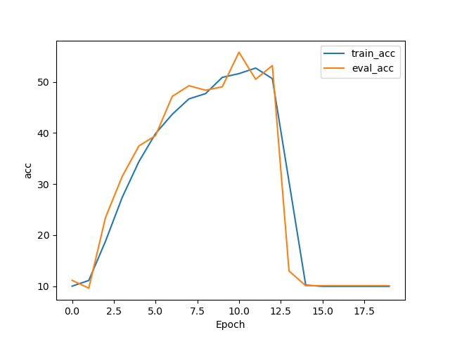
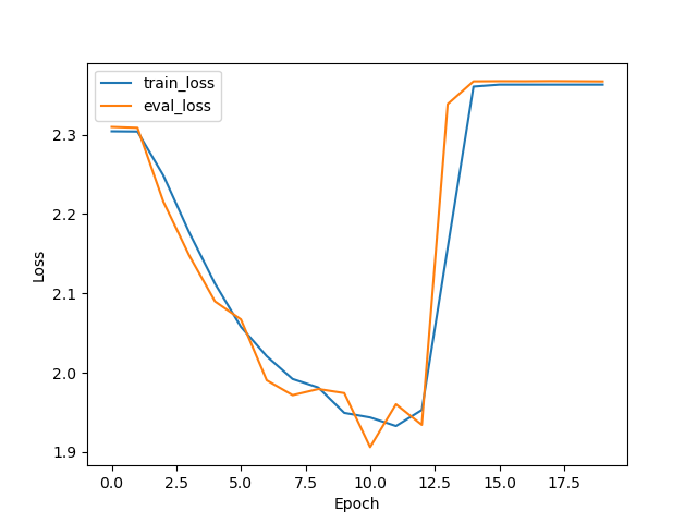
绘制图表 1 2 3 4 5 6 7 8 9 10 11 12 13 fig, ax = plt.subplots() ax.plot(np.arange(args.num_epochs), train_loss, np.arange(args.num_epochs), eval_loss) ax.set_xlabel("Epoch" ) ax.set_ylabel("Loss" ) ax.legend(["train_loss" , "eval_loss" ]) plt.show() fig, ax = plt.subplots() ax.plot(np.arange(args.num_epochs), train_acc, np.arange(args.num_epochs), eval_acc) ax.set_xlabel("Epoch" ) ax.set_ylabel("acc" ) ax.legend(["train_acc" , "eval_acc" ]) plt.show()
softmax 在构建网络的时候,由于没有考虑到交叉熵损失函数中已经包含了 Softmax 函数,而在模型的末尾加入了 Softmax 层,导致网络模型不能正常收敛
Softmax acc-Epoch Softmax Loss-Epoch Torch.nn.CrossEntropyLoss() 函数是先将输出结果输入到 Softmax 层后取对数,再应用 NLLLoss 即 Torch.nn.CrossEntropyLoss() = LogSoftmax + NLLLoss
将模型最后的 Softmax 层去掉网络就可正常收敛了
在此处把警钟敲烂,要和 GPU 一起检查
参考网页 爱学英语的程序媛 - Pytorch划分数据集的方法
Wabi―sabi - AlexNet网络对CIFAR10分类——torch实现
故你, - [pytorch] 利用Alexnet训练cifar10
argparse 库 argparse 可以给 Python 脚本传入参数
使用时需要先导入库
然后实例化参数容器
1 parser = argparse.ArgumentParser()
最后逐一添加所需参数(及其默认值)
1 2 3 parser.add_argument("--gpu" , action="store_true" , default=True , help ="use gpu mode" ) parser.add_argument("--batch_size" , type =int , default=32 , help ="batch size in training" ) parser.add_argument("--num_epochs" , type =int , default=20 , help ="epochs in training" )
后续代码只需要调用 parser 的对应成员即可
参考网页 Fan19zju - argparse库教程(超易懂)